
Introduction
In today’s world of data, the ability to efficiently process and analyze large amount of data is crucial for businesses and organizations. This is where PySpark comes in - an open-source, distributed computing framework built on top of Apache Spark. With its seamless integration with Python, PySpark allows users to leverage the powerful data processing capabilities of Spark directly from Python scripts.
This post was originally a Jupyter Notebook I created when I started learning PySpark, intended as a cheat sheet for me when working with it. As I started to have a blog (a place for my notes), I decided to update and share it here as a complete hands-on tutorial for beginners.
If you are new to PySpark, this tutorial is for you. We will cover the basic, most practical, syntax of PySpark. By the end of this tutorial, you will have a solid understanding of PySpark and be able to use Spark in Python to perform a wide range of data processing tasks.
Spark vs PySpark
What is PySpark? How is it different from Apache Spark? Before looking at PySpark, it’s essential to understand the relationship between Spark and PySpark.
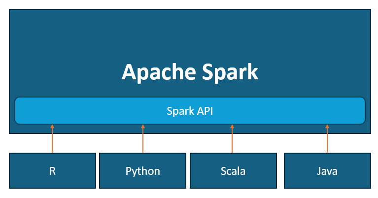
Apache Spark is an open source distributed computing system. It provides an interface for programming clusters with implicit data parallelism and fault tolerance. Apache Spark provides API for various programming languages, including Python, Java, Scala, R, making it accessible to various audiences to perform data processing tasks.
PySpark, on the other hand, is the library that uses the provided APIs to provide Python support for Spark. It allows developers to use Python, the most popular programming language in the data community, to leverage the power of Spark without having to switch to another language. PySpark also offers seamless integration with other Python libraries.
In short, Spark is the overarching framework, PySpark serves as its Python API, providing a convenient bridge for Python enthusiasts to leverage Spark’s capabilities.
Let’s get started
From this point on, you will see Python code doing Spark. This hands-on tutorial will guide you through basic PySpark operations such as querying, filtering, merging, and grouping data. You can find an executable notebook on my Github.
Installation
There are several ways to install PySpark. The easiest way for Python users is to use pip.
pip install pyspark
SparkSession
SparkSession is the entry point for working with Apache Spark. It provides a unified interface for interacting with Spark functionality, allowing you to create DataFrames, execute SQL queries, and manage Spark configurations. Think of it as the gateway to all Spark operations in your application.
from pyspark.sql import SparkSession

# Get existed or Create new SparkSession
spark = SparkSession.builder.appName('Spark Demo').master('local[*]').getOrCreate()
spark
SparkSession - in-memory

SparkContext

Spark UI

Version    v3.2.1
Master     local[*]
AppName    Spark Demo
Load data
PySpark can load data from various types of data storage. In this tutorial we will use the Fraudulent Transactions Dataset. This dataset provides a CSV file that is sufficient for demo purposes.
The SparkSession object provides read as a property that returns a DataFrameReader that can be used to read data as a DataFrame. The following code reads a csv file into a DataFrame.
# Load CSV file to DataFrame
data_path = '../input/fraudulent-transactions-data/Fraud.csv'
df = spark.read.csv(data_path, header=True, inferSchema=True)
df.printSchema()
root
 |-- step: integer (nullable = true)
 |-- type: string (nullable = true)
 |-- amount: double (nullable = true)
 |-- nameOrig: string (nullable = true)
 |-- oldbalanceOrg: double (nullable = true)
 |-- newbalanceOrig: double (nullable = true)
 |-- nameDest: string (nullable = true)
 |-- oldbalanceDest: double (nullable = true)
 |-- newbalanceDest: double (nullable = true)
 |-- isFraud: integer (nullable = true)
 |-- isFlaggedFraud: integer (nullable = true)
The inferSchema parameter allows Spark to automatically infer the data types of each column based on the actual data in the file. This involves reading a sample of data, which can be computationally expensive. This can also be incorrect, especially if sample data doesn’t represent the entire dataset well.
Alternatively, to achieve better performance and ensure accurate data types, you can define the schema explicitly.
from pyspark.sql import types as T

# Read CSV with pre-defined schema
predefined_schema = T.StructType([
    T.StructField('step', T.IntegerType()),
    T.StructField('type', T.StringType()),
    T.StructField('amount', T.DoubleType()),
    T.StructField('nameOrig', T.StringType()),
    T.StructField('oldbalanceOrg', T.DoubleType()),
    T.StructField('newbalanceOrig', T.DoubleType()),
    T.StructField('nameDest', T.StringType()),
    T.StructField('oldbalanceDest', T.DoubleType()),
    T.StructField('newbalanceDest', T.DoubleType()),
    T.StructField('isFraud', T.IntegerType()),
    T.StructField('isFlaggedFraud', T.IntegerType())
])

df = spark.read.csv(data_path, schema=predefined_schema, header=True)
root
 |-- step: integer (nullable = true)
 |-- type: string (nullable = true)
 |-- amount: double (nullable = true)
 |-- nameOrig: string (nullable = true)
 |-- oldbalanceOrg: double (nullable = true)
 |-- newbalanceOrig: double (nullable = true)
 |-- nameDest: string (nullable = true)
 |-- oldbalanceDest: double (nullable = true)
 |-- newbalanceDest: double (nullable = true)
 |-- isFraud: integer (nullable = true)
 |-- isFlaggedFraud: integer (nullable = true)
The data set contains some misformatted column names. I will rename them all to camel case.
# Rename columns
corrected_cols = {'oldbalanceOrg': 'oldBalanceOrig', 'newbalanceOrig': 'newBalanceOrig',
                  'oldbalanceDest': 'oldBalanceDest', 'newbalanceDest': 'newBalanceDest'}
for old_col, new_col in corrected_cols.items():
    df = df.withColumnRenamed(old_col, new_col)

df.printSchema()
root
 |-- step: integer (nullable = true)
 |-- type: string (nullable = true)
 |-- amount: double (nullable = true)
 |-- nameOrig: string (nullable = true)
 |-- oldBalanceOrig: double (nullable = true)
 |-- newBalanceOrig: double (nullable = true)
 |-- nameDest: string (nullable = true)
 |-- oldBalanceDest: double (nullable = true)
 |-- newBalanceDest: double (nullable = true)
 |-- isFraud: integer (nullable = true)
 |-- isFlaggedFraud: integer (nullable = true)
Data Overview
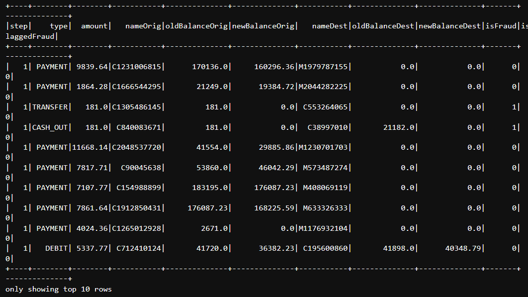
You can quickly look at the data with DataFrame.show which prints the first n rows to the screen.
# Prints top 10 rows of PySpark DataFrame to the screen
df.show(10)
+----+--------+--------+-----------+--------------+--------------+-----------+--------------+--------------+-------+--------------+
|step|    type|  amount|   nameOrig|oldBalanceOrig|newBalanceOrig|   nameDest|oldBalanceDest|newBalanceDest|isFraud|isFlaggedFraud|
+----+--------+--------+-----------+--------------+--------------+-----------+--------------+--------------+-------+--------------+
|   1| PAYMENT| 9839.64|C1231006815|      170136.0|     160296.36|M1979787155|           0.0|           0.0|      0|             0|
|   1| PAYMENT| 1864.28|C1666544295|       21249.0|      19384.72|M2044282225|           0.0|           0.0|      0|             0|
|   1|TRANSFER|   181.0|C1305486145|         181.0|           0.0| C553264065|           0.0|           0.0|      1|             0|
|   1|CASH_OUT|   181.0| C840083671|         181.0|           0.0|  C38997010|       21182.0|           0.0|      1|             0|
|   1| PAYMENT|11668.14|C2048537720|       41554.0|      29885.86|M1230701703|           0.0|           0.0|      0|             0|
|   1| PAYMENT| 7817.71|  C90045638|       53860.0|      46042.29| M573487274|           0.0|           0.0|      0|             0|
|   1| PAYMENT| 7107.77| C154988899|      183195.0|     176087.23| M408069119|           0.0|           0.0|      0|             0|
|   1| PAYMENT| 7861.64|C1912850431|     176087.23|     168225.59| M633326333|           0.0|           0.0|      0|             0|
|   1| PAYMENT| 4024.36|C1265012928|        2671.0|           0.0|M1176932104|           0.0|           0.0|      0|             0|
|   1|   DEBIT| 5337.77| C712410124|       41720.0|      36382.23| C195600860|       41898.0|      40348.79|      0|             0|
+----+--------+--------+-----------+--------------+--------------+-----------+--------------+--------------+-------+--------------+
only showing top 10 rows
In many cases, the result does not fit on the screen and produces unreadable output.
This is where Python comes in. With PySpark, you can mix Python code with Spark APIs to improve the result. The following Python function will show you how to use a Python loop to split and display a sample of data.
# Split columns into subsets and show it accordingly
def show_split(df, split=-1, n_samples=10):
    n_cols = len(df.columns)
    if split <= 0:
        split = n_cols
    i = 0
    j = i + split
    while i < n_cols:
        df.select(*df.columns[i:j]).show(n_samples)
        i = j
        j = i + split

show_split(df, 4, 10)
+----+--------+--------+-----------+
|step|    type|  amount|   nameOrig|
+----+--------+--------+-----------+
|   1| PAYMENT| 9839.64|C1231006815|
|   1| PAYMENT| 1864.28|C1666544295|
|   1|TRANSFER|   181.0|C1305486145|
|   1|CASH_OUT|   181.0| C840083671|
|   1| PAYMENT|11668.14|C2048537720|
|   1| PAYMENT| 7817.71|  C90045638|
|   1| PAYMENT| 7107.77| C154988899|
|   1| PAYMENT| 7861.64|C1912850431|
|   1| PAYMENT| 4024.36|C1265012928|
|   1|   DEBIT| 5337.77| C712410124|
+----+--------+--------+-----------+
only showing top 10 rows

+--------------+--------------+-----------+--------------+
|oldBalanceOrig|newBalanceOrig|   nameDest|oldBalanceDest|
+--------------+--------------+-----------+--------------+
|      170136.0|     160296.36|M1979787155|           0.0|
|       21249.0|      19384.72|M2044282225|           0.0|
|         181.0|           0.0| C553264065|           0.0|
|         181.0|           0.0|  C38997010|       21182.0|
|       41554.0|      29885.86|M1230701703|           0.0|
|       53860.0|      46042.29| M573487274|           0.0|
|      183195.0|     176087.23| M408069119|           0.0|
|     176087.23|     168225.59| M633326333|           0.0|
|        2671.0|           0.0|M1176932104|           0.0|
|       41720.0|      36382.23| C195600860|       41898.0|
+--------------+--------------+-----------+--------------+
only showing top 10 rows

+--------------+-------+--------------+
|newBalanceDest|isFraud|isFlaggedFraud|
+--------------+-------+--------------+
|           0.0|      0|             0|
|           0.0|      0|             0|
|           0.0|      1|             0|
|           0.0|      1|             0|
|           0.0|      0|             0|
|           0.0|      0|             0|
|           0.0|      0|             0|
|           0.0|      0|             0|
|           0.0|      0|             0|
|      40348.79|      0|             0|
+--------------+-------+--------------+
only showing top 10 rows
When working with numerical data, it is not very useful to look at a long series of values. We are often more interested in a few key information points, such as count, mean, standard deviation, minimum, and maximum. PySpark’s DataFrame provides describe and summary function with different usage to present these essential metrics.
# DataFrame.describe take columns as params
df.describe('step', 'amount').show()
+-------+------------------+------------------+
|summary|              step|            amount|
+-------+------------------+------------------+
|  count|           6362620|           6362620|
|   mean|243.39724563151657|179861.90354913412|
| stddev|142.33197104912588| 603858.2314629498|
|    min|                 1|               0.0|
|    max|               743|     9.244551664E7|
+-------+------------------+------------------+
# DataFrame.summary take statistics as params
df.select('oldBalanceOrig', 'newBalanceOrig', 'oldBalanceDest', 'newBalanceDest').summary('count', 'min', 'max', 'mean', '50%').show()
+-------+-----------------+-----------------+------------------+------------------+
|summary|   oldBalanceOrig|   newBalanceOrig|    oldBalanceDest|    newBalanceDest|
+-------+-----------------+-----------------+------------------+------------------+
|  count|          6362620|          6362620|           6362620|           6362620|
|    min|              0.0|              0.0|               0.0|               0.0|
|    max|    5.958504037E7|    4.958504037E7|    3.5601588935E8|    3.5617927892E8|
|   mean|833883.1040744719|855113.6685785714|1100701.6665196654|1224996.3982019408|
|    50%|         14211.23|              0.0|         132612.49|         214605.81|
+-------+-----------------+-----------------+------------------+------------------+
Query data
Select and Filter
PySpark borrowed a lot of vocabulary from the SQL world. But it offers the flexibility that we do not need to follow the strict SQL framework (select … from … where …). Each step of PySpark will return a DataFrame or GroupedData that we can continue to work with normally.
from pyspark.sql import functions as F

# First .where() filter DataFrame and return another DataFrame
# Then .select() select from the returned DataFrame
df.where(df['type']=='CASH_OUT').select(df.type, F.col('amount')).show(10)
+--------+---------+
|    type|   amount|
+--------+---------+
|CASH_OUT|    181.0|
|CASH_OUT|229133.94|
|CASH_OUT|110414.71|
|CASH_OUT|  56953.9|
|CASH_OUT|  5346.89|
|CASH_OUT|  23261.3|
|CASH_OUT| 82940.31|
|CASH_OUT| 47458.86|
|CASH_OUT|136872.92|
|CASH_OUT| 94253.33|
+--------+---------+
only showing top 10 rows
The above example shows us three different ways to access pyspark columns:
df.type: Access as an attribute.df['type']: Access as an items.F.col('type'): Explicitly specify that we need a column, not a string literal.
You can also filter multiple conditions using &, |, and ~ operator.
# PySpark example filter multiple conditions
df.where((F.col('type')=='CASH_OUT') & (F.col('amount') > 500)).show(10)
For users who are more familiar with SQL syntax, Spark provides the ability to write SQL queries directly. Before writing SQL queries in PySpark, you need to register your DataFrame. This allows you to reference it in your SQL queries.
# Create or replace temp view named "df" from DataFrame df in PySpark
df.createOrReplaceTempView('df')

# Spark SQL query example. You can now reference df in your query
spark.sql('''
    SELECT type, amount
    FROM df
    WHERE type = "CASH_OUT"
''').show(10)
+--------+---------+
|    type|   amount|
+--------+---------+
|CASH_OUT|    181.0|
|CASH_OUT|229133.94|
|CASH_OUT|110414.71|
|CASH_OUT|  56953.9|
|CASH_OUT|  5346.89|
|CASH_OUT|  23261.3|
|CASH_OUT| 82940.31|
|CASH_OUT| 47458.86|
|CASH_OUT|136872.92|
|CASH_OUT| 94253.33|
+--------+---------+
only showing top 10 rows
Aggregating with groupBy
PySpark provides a similar syntax to Pandas for aggregating data.
# Example to PySpark groupBy
# Sometimes we can pass column name directly to pyspark functions
# `Column.alias` method change the name of the result column.
df.select('type', 'amount').groupBy('type').agg(F.mean('amount').alias('avgAmount')).orderBy('avgAmount').show(10)
spark.sql('''
    SELECT type, AVG(amount) avgAmount
    FROM df
    GROUP BY type
    ORDER BY 2
''').show(10)
+--------+------------------+
|    type|         avgAmount|
+--------+------------------+
|   DEBIT| 5483.665313767128|
| PAYMENT|13057.604660187604|
| CASH_IN| 168920.2420040954|
|CASH_OUT|176273.96434613998|
|TRANSFER| 910647.0096454868|
+--------+------------------+
To filter after groupBy, we can just simply apply where or filter to the result DataFrame object or follow SQL framework with having keyword.
(
    df.where(df['type']=='CASH_OUT')
    .groupBy('nameOrig')
    .agg(F.sum('amount').alias('sumAmount'))
    .where(F.col('sumAmount') > 300000)
    .show(10)
)
spark.sql('''
    SELECT nameOrig, SUM(amount) sumAmount
    FROM df
    WHERE type = "CASH_OUT"
    GROUP BY 1
    HAVING sumAmount > 300000
''').show(10)
+-----------+---------+
|   nameOrig|sumAmount|
+-----------+---------+
| C551314014|301050.58|
| C661668091|323789.56|
| C228994633|517946.01|
|C1591008292|558254.22|
|C2100435651|357988.09|
| C624052656|476735.47|
| C948681098|353759.28|
|  C50682517|386128.82|
|C1579521009|684561.18|
|C1871922377|394317.12|
+-----------+---------+
only showing top 10 rows
Union and Intersection
df.select('nameOrig').union(df.select('nameDest')).count()
12725240
spark.sql('''
    SELECT nameOrig from df
    UNION
    SELECT nameDest from df
''').count()
9073900
We can see the difference in the count here. The reason is that PySpark union function keeps the duplicate samples from two sets. This is equivalent to UNION ALL in SQL. By default, PySpark will not remove duplidates as it is an expensive process. If you want to drop duplicates, you have to do it explicitly.
# Union and drop duplicates in PySpark
df.select('nameOrig').union(df.select('nameDest')).dropDuplicates().count()
9073900
Unioning can be useful when we are reading data from multiple files. We can read them one by one in a Python loop and union them.
Intersection is similar to Union. But, keep in mind that PySpark intersect is equivalent to SQL INTERSECT, not INTERSECT ALL.
Join
Very similar to Pandas, DataFrame.join method joins a DataFrame with another DataFrame using the given join expression.
(
    df.where('type = "CASH_IN" OR type = "CASH_OUT"')
    .selectExpr('nameOrig', 'ABS(newBalanceOrig - oldBalanceOrig) changeOrig')
    .groupBy('nameOrig')
    .agg(
        F.mean(F.col('changeOrig')).alias('avgChangeOrig'),
        F.count('*').alias('occOrig')
    )
    .where('avgChangeOrig > 100000')
    # Join the above DataFrame with the one provided in parameter
    .join((
        df.where('type = "CASH_IN" OR type = "CASH_OUT"')
        .selectExpr('nameDest', 'ABS(newBalanceDest - oldBalanceDest) changeDest')
        .groupBy('nameDest')
        .agg(
            F.mean(F.col('changeDest')).alias('avgChangeDest'),
            F.count('*').alias('occDest')
        )
        .where('avgChangeDest > 100000')
    ), on=F.col('nameOrig')==F.col('nameDest'), how='inner')
    # There are several join method: inner, left, right, cross, outer, left_outer, right_outer, left_semi, left_anti, right_semi, right_anti, ...
    .selectExpr('nameOrig name', 'occOrig + occDest occ', 'avgChangeOrig', 'avgChangeDest')
    .orderBy('occ', ascending=False)
).show(10)
spark.sql('''
    SELECT nameOrig name, occOrig + occDest occ, avgChangeOrig, avgChangeDest
    FROM
    (
        SELECT nameOrig, AVG(ABS(newBalanceOrig - oldBalanceOrig)) avgChangeOrig, COUNT(*) occOrig
        FROM df
        WHERE type = "CASH_IN" OR type = "CASH_OUT"
        GROUP BY nameOrig
        HAVING avgChangeOrig > 100000
    )
    INNER JOIN
    (
        SELECT nameDest, AVG(ABS(newBalanceDest - oldBalanceDest)) avgChangeDest, COUNT(*) occDest
        FROM df
        WHERE type = "CASH_IN" OR type = "CASH_OUT"
        GROUP BY nameDest
        HAVING avgChangeDest > 100000
    )
    ON nameOrig = nameDest
    ORDER BY occ DESC
''').show(10)
+-----------+---+------------------+------------------+
|       name|occ|     avgChangeOrig|     avgChangeDest|
+-----------+---+------------------+------------------+
|C1552859894| 43|193711.30000000005| 763241.1652380949|
|C1819271729| 37|         278937.79|283626.17805555544|
|C1692434834| 37|177369.73000000045| 438853.7616666666|
| C889762313| 32|         132731.31|211437.18741935486|
|C1868986147| 32|         120594.03|249840.37709677417|
|  C55305556| 28|319860.45999999903|225565.42111111112|
| C636092700| 26|217273.86000000004|201888.05279999998|
|C1713505653| 25| 278622.8400000003|186625.34916666665|
|C2029542508| 24| 235760.1200000001|231022.98217391354|
| C699906968| 23| 177813.3799999999| 183054.3072727272|
+-----------+---+------------------+------------------+
only showing top 10 rows
In the above example, I demonstrated mixing Python Spark and SQL syntax for cleaner code. Instead of the verbose expression:
df.where((F.col('type')=='CASH_IN') | (F.col('type')=='CASH_OUT'))
You can write:
df.where('type = "CASH_IN" OR type = "CASH_OUT"')
This style can be applied in various Python Spark functions: selectExpr, where, filter, expr,… Choose your preferred coding style – PySpark offers the flexibility.
Endnote
This tutorial has covered basic Spark operations in both Python and SQL syntax. You will be able to perform most common data transformation and analysis tasks. But your Spark journey doesn’t end here! There are more advanced features that were not covered in this article (e.g., UDF). They will be discussed in another post soon.